Algoim is a collection of high-order accurate numerical methods and C++ algorithms for working with implicitly-defined geometry and level set methods. It includes:
- High-order accurate quadrature algorithms for computing integrals over implicitly-defined domains. Two different approaches are provided:
- Quadrature methods for domains implicitly-defined by a single level set function (sufficiently-smooth, but otherwise arbitrary); and
- Quadrature methods for multi-component domains implicitly-defined by multivariate polynomials, handling complex geometry such as multiple high-curvature pieces, junctions, self-intersections, and cusps.
- High-order accurate algorithms for computing closest points on implicitly-defined surfaces, with application to high-order level set reinitialisation and extension velocity schemes.
- k-d trees optimised for codimension-one point clouds.
Contents
- Prerequisites
- Download
- Installation
- High-Order Quadrature Algorithms for Implicitly-Defined Domains
- High-Order Algorithms for Computing Closest Points on Implicitly-Defined Surfaces
- k-d Trees Optimised for Codimension-One Point Clouds
- Advanced: High-Precision Arithmetic
- About
Prerequisites
A C++ compiler supporting the C++17 standard or higher is required. In addition, if you want to use the quadrature algorithms for domains implicitly-defined by multivariate polynomials, a LAPACKE implementation is required (or a suitable alternative, e.g., Eigen).
Download
Clone via
git clone https://github.com/algoim/algoim.git
or visit the Algoim GitHub page.
Installation
Algoim is a header-only C++ library. Except for small example/demonstration applications, all of the files are C++ .hpp header files. As such, it requires minimal installation effort: simply download and configure so that the appropriate header driver can be found by your compiler when you include it in your C++ program, e.g., #include "algoim/quadrature_general.hpp".
High-Order Quadrature Algorithms for Implicitly-Defined Domains
An implicitly-defined domain is a volumetric region or codimension-one surface whose shape is defined implicitly by an isosurface of one or more scalar functions. Algoim implements two kinds of quadrature algorithms for computing integrals over implicitly-defined domains:
- The first technique targets general, sufficiently smooth level set functions, and is based on the paper R. I. Saye, High-Order Quadrature Methods for Implicitly Defined Surfaces and Volumes in Hyperrectangles, SIAM Journal on Scientific Computing, 37(2), A993-A1019 (2015).
- The second technique targets level set functions defined by one or more multivariate polynomials, and is based on the paper R. I. Saye, High-order quadrature on multi-component domains implicitly defined by multivariate polynomials, Journal of Computational Physics, 448, 110720 (2022).
Both techniques operate by reinterpreting the implicitly-defined geometry as the graph of an implicitly-defined (potentially multi-valued) height function, followed by a dimension-reduction approach and one-dimensional quadrature methods. Both techniques construct quadrature schemes with positive weights and can yield high-order accuracy; e.g., with 4 points per one-dimensional line integral, 8th order accuracy can be achieved (for sufficiently nice geometry).
The following table may help guide you in choosing between these two techniques.
| Implicitly-defined domain specified by a single level set function, sufficiently-smooth but otherwise arbitrary | Implicitly-defined domain specified by one or more multivariate polynomials |
|---|---|
| Applicable to any level set function for which “Interval” arithmetic can be applied (roughly speaking, any function for which you can compute a first-order Taylor series and sufficiently bound the remainder; see below). | Applicable only to level set function(s) defined by multivariate polynomials, generally of small-to-medium degree. |
| Works best when the implicitly-defined interface can be viewed as the graph of a well-defined, sufficiently smooth height function, e.g., no isolated droplets, corners, or singularities; applies heuristic subdivision methods whenever this is not the case. | Can handle complex geometry, e.g., multi-component domains, high-curvature pieces, tunnels, junctions, self-intersections, and cusps; subdivision methods are not needed. |
| In the simplest case, assumes the domain is constrained by a user-defined hyperrectangle. | Can be used on hyperrectangular and simplex constraint cells; in fact, any compact semi-algebraic set constraint domain is possible. |
| On very smooth geometry, generally very fast, with small node counts; on very complex geometry, can result in large node counts. | On small-to-medium degree polynomials, generally very fast, with small node counts (even for complex geometry); high-degree polynomials and/or high dimensions can be slower and more ill-conditioned. |
Some examples illustrating the quadrature schemes are shown in the next two sections.
Quadrature algorithms for general, sufficiently smooth level set functions
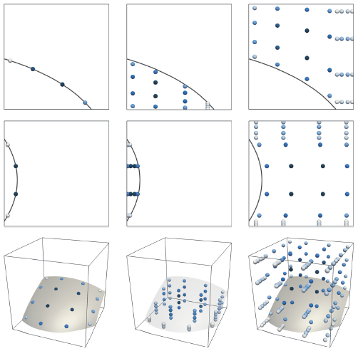
Some examples illustrating the quadrature schemes constructed by the algorithm (based on a one-dimensional Gaussian quadrature scheme of node-count 4) for surface integrals (left column) and volume integrals (middle/right columns). The weights are coloured according to a scale that is normalised for each particular case: pale indicates a low-valued weight and dark blue indicates a high-valued weight.
The driver header file for these quadrature algorithms is located at algoim/quadrature_general.hpp. There is only one driver routine, quadGen which is templated on the level set function object phi and the dimension N:
template<int N, typename F>
algoim::QuadratureRule<N> algoim::quadGen(const F& phi, const algoim::HyperRectangle<real,N>& xrange, int dim, int side, int qo);
The parameters are as follows:
phiis a user-defined function object which evaluates the level set function and its gradient. It must implement bothtemplate<typename T> operator() (const algoim::uvector<T,N>& x) constandtemplate<typename T> grad(const algoim::uvector<T,N>& x) const. In the simplest case,T = doubleand the role ofphiis to simply evaluate the level set function (e.g.,return x(0)*x(0) + x(1)*x(1) - 1;for a unit circle) and its gradient (e.g.,return algoim::uvector<double,2>(2*x(0), 2*x(1));). However, it is crucial that these two member functions be templated onTto enable interval arithmetic. In essence, the interval arithmetic automatically computes a first-order Taylor series (with bounded remainder) of the given level set function, and uses that to make decisions concerning the existence of the interface and what direction to use when converting the implicitly-defined geometry into the graph of an implicitly-defined height function. This requirement onphibeing able to correctly perform interval arithmetic places restrictions on the type of level set functionsquadGencan be applied to; these restrictions are discussed later.xrangeis a user-specified bounding box, indicating the extent of theN-dimensional constraint cell.dimis used to specify the type of quadrature:- If
dim < 0, compute a volumetric quadrature scheme, whose domain is implicitly defined by{phi < 0}intersected withxrange. - If
dim == N, compute a curved surface quadrature scheme, whose domain is implicitly defined by{phi = 0}intersected withxrange. - If
0 <= dim && dim < N, compute a flat surface quadrature scheme for one of the sides of the hyperrectangle, i.e., for the domain{phi < 0}, intersected withxrange, intersected with the flat face{x(dim) == xrange.side(side)(dim)}.
- If
sideis used only when0 <= dim && dim < Nand specifies which side of the hyperrectangle to restrict to, eitherside == 0orside == 1for the “left” or “right” face, respectively (with normal pointing in the direction of thedim-th axis).qospecifies the degree of the underlying one-dimensional Gaussian quadrature scheme and must satisfy1 <= qo && qo <= 100. For example,qo = 4in the figure above.
The output of quadGen is an algoim::QuadratureRule<N> object. This object is essentially a std::vector listing the set of quadrature points and their corresponding weights. A QuadratureRule object is also a functor – its associated templated member function operator()(const F& f) can be applied to any user-specified integrand function to compute the result of applying the quadrature rule to a functional.
Requirements on phi. As mentioned above, the phi functor must be able to accept arguments of type algoim::uvector<algoim::Interval<N>,N>. Here, algoim::Interval<N> is a special type whose purpose is to calculate a first-order Taylor series with bounded remainder, similar to automatic differentiation (see the paper cited above for more details). Interval<N> implements operator+, operator*, operator/, etc., and can be used in a variety of ways, most commonly in evaluating simple algebraic expressions. Common unary operators are also implemented, e.g., sin(Interval<N>) and exp(Interval<N>). However, one cannot straightforwardly apply Interval<N> arithmetic to max or min statements, if conditions, and other non-standard or non-smooth functions. When using Algoim quadrature schemes for the first time, it is recommended they be applied to smooth level set functions made out of polynomial expressions and common smooth functions like sin, exp, etc.
Examples
All of these examples are implemented in examples/examples_quad_general.cpp in a single main() entry point; compile them with a C++17-compatible compiler of your choice.
The quadrature algorithms of Algoim are here demonstrated with a level set function describing an ellipse (in N = 2 dimensions) or ellipsoid (in N = 3 dimensions). First, we define a function object implementing the level set function:
template<int N>
struct Ellipsoid
{
    template<typename T>
    T operator() (const algoim::uvector<T,N>& x) const
    {
        if constexpr (N == 2)
            return x(0)*x(0) + 4.0*x(1)*x(1) - 1.0;
        else
            return x(0)*x(0) + 4.0*x(1)*x(1) + 9.0*x(2)*x(2) - 1.0;
    }

    template<typename T>
    algoim::uvector<T,N> grad(const algoim::uvector<T,N>& x) const
    {
        if constexpr (N == 2)
            return algoim::uvector<T,N>(2.0*x(0), 8.0*x(1));
        else
            return algoim::uvector<T,N>(2.0*x(0), 8.0*x(1), 18.0*x(2));
    }
};
To compute the area of the ellipse in 2D using a scheme with qo = 4, apply quadGen to a bounding box encapsulating the extent of the ellipse, and then apply the resulting quadrature rule to the integrand f(x) = 1:
Ellipsoid<2> phi;
auto q = algoim::quadGen<2>(phi, algoim::HyperRectangle<double,2>(-1.1, 1.1), -1, -1, 4);
double area = q([](const auto& x) { return 1.0; });
// area ≈ 1.5708
To compute the volume of the ellipsoid in 3D, simply change N:
Ellipsoid<3> phi;
auto q = algoim::quadGen<3>(phi, algoim::HyperRectangle<double,3>(-1.1, 1.1), -1, -1, 4);
double volume = q([](const auto& x) { return 1.0; });
// volume ≈ 0.69813
Each of the two examples above relied on the quadrature scheme’s ability to automatically subdivide the given bounding box until the interface geometry can be represented as the graph of a well-defined, single-valued height function. The subdivision routine terminates as soon as an internal criterion is met (discussed more in the paper cited above). An alternative method revealing asymptotic high-order accuracy (under h-refinement) is to subdivide the ellipsoid via a Cartesian grid and apply quadGen to individual grid cells, as follows:
int n = 16;
double dx = 2.2 / n;
Ellipsoid<2> phi;
double area = 0.0;
for (int i = 0; i < n; ++i) for (int j = 0; j < n; ++j)
{
    algoim::uvector<double,2> xmin{-1.1 + i*dx, -1.1 + j*dx};
    algoim::uvector<double,2> xmax = xmin + dx;
    area += algoim::quadGen<2>(phi, algoim::HyperRectangle<double,2>(xmin, xmax), -1, -1, 4).sumWeights();
}
// area ≈ 1.570796327
To compute the measure of an implicitly-defined codimension-one surface, change the dim parameter to equal N:
Ellipsoid<3> phi;
auto q = algoim::quadGen<3>(phi, algoim::HyperRectangle<double,3>(-1.1, 1.1), 3, -1, 4);
double surface_area = q.sumWeights();
// surface_area ≈ 4.4007
To visualise a quadrature scheme produced by algoim::quadGen, one possibility is to use the tool provided in algoim/quadrature_general.hpp. This method outputs a scheme in the format of an XML VTK .vtp file, which you can open with, e.g., ParaView. The routine takes as input a user-defined stream (e.g., a std::ofstream) and writes XML to the stream, interpreting the quadrature scheme as a scattered set of points with associated weights:
#include <fstream>
...
algoim::QuadratureRule<N> q = ...;
std::ofstream f("scheme.vtp");
algoim::outputQuadratureRuleAsVtpXML(q, f);
// Open 'scheme.vtp' in ParaView
Citing
If you make use of these quadrature algorithms in your work, in any documentation or publication please cite the following paper. Doing so is a nice way to credit me (and my sponsors) for the time and resources it took to develop and publish this code.
Quadrature algorithms for domains implicitly-defined by multivariate polynomials
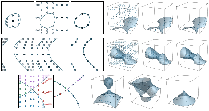
Some examples illustrating the quadrature schemes constructed by the algorithm (based on a one-dimensional Gaussian quadrature scheme of node-count 3). Each of the four examples in the top two rows illustrate the quadrature scheme for the inside, outside, and surface. The bottom-left example illustrates a case of two intersecting polynomials whose interfaces meet at a junction; the quadrature scheme is high-order accurate on each component (indicated by the colours). The bottom-right examples illustrate 3D cases with singularities, such as cusps and self-intersections.
The driver header file for these quadrature algorithms is located at algoim/quadrature_multipoly.hpp. These methods are templated on the dimension N, and algoim::ImplicitPolyQuadrature<N> implements the core driver. To build a quadrature scheme, there are essentially three steps:
- Instantiate a multivariate Bernstein polynomial, one for each level set function. In Algoim, these are implemented as tensor-product Bernstein polynomials, whose coefficients are stored in
N-dimensional arrays. These arrays are manipulated viaalgoim::xarrayobjects (representing a view to a contiguous blockalgoim::reals), whilealgoim/bernstein.hppimplements several routines for manipulating Bernstein polynomials. One of the simplest approaches to instantiate anN-dimensional Bernstein polynomial is to use thealgoim::bernstein::bernsteinInterpolate<N>method, which outputs the unique polynomial interpolating the given functor at the nodes of a Chebyshev-based tensor-product grid. - Next, create an
algoim::ImplicitPolyQuadrature<N>object with the above Bernstein polynomials as input parameters. The creation of theImplicitPolyQuadratureobject executes the hierarchical construction phase of the quadrature algorithm: in essence, a height direction is automatically chosen and the implicitly-defined integral is recast as a base integral (in one fewer dimensions) of a one-dimensional integrand, continuing recursively down to theN = 1base case. For details, see the paper. - After building the hierarchy, call
integrate(for volumetric integrals) orintegrate_surf(for surface integrals), with parameters specifying the one-dimensional node count q and the integrand f. The latter is a function object implementingoperator() (const algoim::uvector<real,N>& x, algoim::real w), taking the quadrature node and weight as input. For example, f can be used to record the given quadrature points, e.g., for later usage in a finite element method, or for visualisation purposes.
Example
As a simple example, suppose you wanted to build a quadrature scheme for a 3D ellipsoid. First, define a functor which returns the (polynomial) level set function value:
auto ellipsoid = [](const uvector<real,3>& x)
{
    return x(0)*x(0) + x(1)*x(1)*4 + x(2)*x(2)*9 - 1;
};
Second, set aside some memory to store the coefficient values of a tensor-product Bernstein polynomial, which in this case would be a triquadratic polynomial requiring 27 scalar values:
real data[27]; // or some other memory block elsewhere, on the stack, heap, etc.
xarray<real,3> phi(data, uvector<int,3>(3,3,3)); // (3,3,3) indicates the array extent, equal to the Bernstein degree plus one
Third, build the Bernstein coefficients corresponding to the ellipsoid level set function. There are many ways to do this, e.g., converting the coefficients in a monomial basis to the Bernstein basis or solving an interpolation problem. In many circumstances, the interpolation method provided in algoim/bernstein.hpp is a convenient approach:
bernstein::bernsteinInterpolate<N>([&](const uvector<real,N>& x) { return ellipsoid(xmin + x * (xmax - xmin)); }, phi);
The coordinate system of bernstein::bernsteinInterpolate is relative to the unit cube [0,1]N; these coordinates are then mapped to custom domain [xmin,xmax] when evaluating the ellipsoid functor. Having built the input Bernstein polynomial, we can then build the quadrature hierarchy:
ImplicitPolyQuadrature<3> ipquad(phi);
and then build a volumetric quadrature scheme as follows:
int q = 3; // q nodes per one-dimensional line integral
std::vector<uvector<real,N>> phase0, phase1; // stores quadrature nodes for the 'inside' and 'outside'
ipquad.integrate(AutoMixed, q, [&](const uvector<real,N>& x, real w)
{
    if (bernstein::evalBernsteinPoly(phi, x) < 0)
        phase0.push_back(x);
    else
        phase1.push_back(x);
});
In the above code, the integrate method is given a lambda which records the quadrature point in the vectors phase0 and phase1, depending on whether the quadrature point is inside or outside the ellipsoid, respectively. Meanwhile, the AutoMixed parameter controls the quadrature strategy; see the in-depth discussion of the paper as well as the comments given in algoim/quadrature_multipoly.hpp.
Additional examples
Additional examples are given in examples/examples_quad_multiply.cpp in a single main() entry point; compile them with a C++17-compatible compiler of your choice. The examples include:
- q-convergence tests, examining the error as the quadrature node count increases,
- replication of some of the examples shown in the paper.
Citing
If you make use of these quadrature algorithms in your work, in any documentation or publication please cite the following paper. Doing so is a nice way to credit me (and my sponsors) for the time and resources it took to develop and publish this code.
High-Order Algorithms for Computing Closest Points on Implicitly-Defined Surfaces
A powerful technique for representing curves in two dimensions (N = 2) and surfaces in three dimension (N = 3) is to define them implicitly as a level set of a continuous, N-dimensional scalar function. This technique of embedding the surface geometry in a higher-dimensional function (which is often called the “level set function”) leads to a wide array of mathematical and computational advantages, as exemplified by the level set method for moving interface problems, and the Voronoi implicit interface method for computing multiphase interface evolution.
Numerical methods making use of this idea often require accurate approximations of nearest points on implicitly-defined surfaces. High-order accurate algorithms for this purpose are described in the paper R. I. Saye, High-order methods for computing distances to implicitly defined surfaces, Communications in Applied Mathematics and Computational Science, 9(1), 107-141 (2014) (pdf copy is provided here).
Provided in Algoim is C++ code implementing the algorithms developed in the paper. These algorithms can be used to implement, for example, high-order accurate reinitialisation/redistancing algorithms in level set methods. The code mainly applies to the case that the level set function is defined on a rectangular Cartesian grid. However, as discussed in the paper, it is possible to extend the algorithms to the case of unstructured grids - one could use the code as a starting point. For example, the implementations of the k-d tree and Newton’s method could be used as-is without modification in such an adaptation.
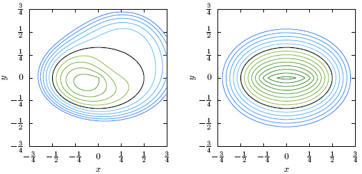
Reinitialising a two-dimensional level set function. (left) Contour plot of a function which implicitly defines an elliptical interface (black curve). (right) Contour plot of the corresponding reinitialised signed distance function.
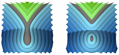
Level sets of a signed distance function reconstructed from the surface shown in grey. This example was constructed from a small 5 by 5 by 5 patch of grid cells, in such a way that the droplet on the right is completely contained within one grid cell. Subgrid details such as this are important in high-order methods involving implicitly-defined geometry.
Usage
The high-order closest point algorithms are located in a number of header files:
algoim/newtoncp.hpp: Newton’s method for the constrained minimum-distance optimisation problem applied to finding closest points on the zero level set of a function (typically a polynomial).algoim/stencilpoly.hpp: Implements the stencil-based polynomial interpolation algorithms for 10 different classes of polynomial in 2D and 3D, including bicubic and tricubic interpolants.algoim/kdtree.hpp: Implements a k-d tree data structure for a given collection of points in RN. This particular k-d tree has been optimised for clouds of points that originate from smooth codimension-one surfaces using coordinate transformations that result in “tight” bounding boxes for nodes in the tree. More details are provided below.algoim/hocp.hpp: Main driver routines for the high-order closest point algorithm applied to rectangular Cartesian grids.
A typical framework using these algorithms operates in two steps. First, in a setup phase, a algoim::KDTree is created based on a cloud of seed points approximately sampling the interface. Second, for a closest point query given a point x, the closest seed point to x is found using the algoim::KDTree and this approximation is then “polished” using Newton’s method (algoim::newtonCP) applied to piecewise polynomial interpolants of the level set function (algoim::StencilPoly<N,Degree> or equivalent).
Examples
These ideas are demonstrated in two example programs. Each cpp file contains a single main() entry point; compile them (individually) with a C++17 compatible compiler of your choice.
examples/examples_hocp_simple.cpp: The code demonstrates a very simple problem of reinitialising a level set function in 2D and 3D. Type in a dimension (2 or 3) and the number of grid points in each axis to have the program reinitialise a spherical interface level set function and report the maximum-norm error of the computed signed distance function.examples/examples_hocp_convergence.cpp: This program implements a series of convergence tests on different interface geometries and can be used to replicate the results in the above cited paper. Use it by specifying the test problem via command-line parameters – for example,./examples_hocp_convergence 2 sphereor./examples_hocp_convergence 3 ellipsoid.
Citing
If you make use of these high-order closest point algorithms in your research, in any documentation or publication please cite the following paper. Doing so is a nice way to credit me (and my sponsors) for the time and resources it took to develop and publish this code.
k-d Trees Optimised for Codimension-One Point Clouds
k-d trees are one of the most effective data structures for finding the closest point in a cloud of scattered points (i.e., a nearest-neighbour search). In its standard form, a k-d tree recursively subdivides the cloud of points along alternating axes. If the point data is situated on or near a smooth codimension-one surface (e.g., a sphere in 3D), the performance of a k-d tree can be further optimised by using approximations of the surface tangent hyperplane. This idea is further detailed in the paper R. I. Saye, High-order methods for computing distances to implicitly defined surfaces, Communications in Applied Mathematics and Computational Science, 9(1), 107-141 (2014) (pdf copy is provided here) and an implementation of the resulting k-d tree optimised for codimension-one point clouds is given in Algoim’s algoim/kdtree.hpp.
An example of its usage is as follows.
#include "algoim/kdtree.hpp"
...
// Generate a random set of points on the surface of a sphere
std::vector<uvector<double,3>> pts;
for (int i = 0; i < 1000; ++i)
{
    uvector<double,3> x(rand(), rand(), rand());
    pts.push_back(x / norm(x));
}
// Build a kdtree of the point cloud
algoim::KDTree<double,3> tree(pts);
// Find the closest point to some query point y
uvector<double,3> y(rand(), rand(), rand());
y /= norm(y);
int ind = tree.nearest(y);
// The closest point is then pts[ind]
Advanced: High-Precision Arithmetic
By default, Algoim is configured to use double-precision arithmetic. For high-precision applications of the associated high-order accurate algorithms, Algoim can interface to a user-defined high-precision scalar type by redefining the algoim::real typedef in algoim/real.hpp. One possibility is to use the open-source QD library which implements software-driven double-double and quadruple-double arithmetic.
To make use of high-precision arithmetic in Algoim, a few modifications may be needed, depending on what part of Algoim is being used:
- Some of the embedded/precomputed numbers may need to be updated. For example, the precomputed Gaussian quadrature schemes in
algoim/gaussquad.hpp, which have about 20 digits of accuracy, would need updating for double-double or quadruple-double accuracy. (I can provide this data to 75 digits of accuracy upon request.) - Regarding the quadrature algorithms for domains implicitly-defined by polynomials, the provided code in Algoim assumes a LAPACKE implementation is available. LAPACK is used for just two purposes: (i) computing SVD factorisations and (ii) solving generalised eigenvalue problems. These methods would need to be replaced with ones supporting high-precision arithmetic. One possibility is to use Eigen. Note: left unmodified, QD is incompatible with Eigen (because of ambiguous overloads when an integer is assigned to a
dd_realorqd_realobject); however it is relatively straightforward to patch QD so that it can work with Eigen. Besides QD there are also several other possibilities for high-precision arithmetic, e.g. Boost.
About
Algoim was developed by Robert Saye in the Mathematics Group at the Lawrence Berkeley National Laboratory as part of his research on numerical methods for high-order accurate interface dynamics, with applications in multi-phase multi-physics. For more information and applications of these algorithms, visit his research page.
This work was supported in part by the U.S. Department of Energy (DOE), Office of Science, Office of Advanced Scientific Computing Research (ASCR) Applied Mathematics Program, by a DOE Office of Science Early Career Research Program award, and by the DOE ASCR Scientific Discovery through Advanced Computing (SciDAC) FASTMath program, all under Contract No. DE-AC02-05CH11231 at Lawrence Berkeley National Laboratory.